The Hong Kong Practitioner

September 2018, Volume 40, No. 3

Update Article

Methodology and statistics for clinical research – Part 1: descriptive statistics

Stanley CN Ha 夏正楠

HK Pract 2018;40:93-96

Summary

To begin a clinical research, we need a lot of statistical knowledge in designing the protocol, selecting the patients, choosing correct statistical tests and drawing valid conclusions. Therefore, the purpose of this article is to give you some basic background knowledge of statistics and the use of statistics to begin a clinical research. The major knowledge you will learn after reading this article includes (1) 4 types of measurement scales (nominal , ordinal , interval and ratio) , (2) difference between dependent and independent variables, (3) normal distribution of a data, population and sample, variance and standard deviation and (4) the way to construct confidence interval.

摘要

當我們開始臨床研究時，我們需要大量的統計知識，包括設計研究大綱，選擇參加者，選擇正確的統計測試和總結有效結論。因此，本文的目的是為你提供一些基本的背景知識了解統計數據，並利用統計學來進行臨床研究。閱讀本文後，你學習的主要知識包括4種數據測量方法（類別(nominal)、等級(ordinal)、等距(interval)和等比(ratio)），獨立變項(independent variable)和依變項(dependent variable)的差異，標準常態分配(normal distribution)，母體(population)和樣本(sample)，標準差(standard deviation)和變異數(variance)，計算信賴區間 (confidence interval)的方法。

Introduction

Statistics is all about probability and distribution. It is a tool to help us analysis clinical research in order to draw a conclusion, which is part of the whole clinical research design. It tells us the relationship among the outcomes, whether there is enough evidence to conclude that the outcomes are different among different groups, how the data distributes, etc. Before going into how to use statistics to do analysis and draw conclusions, some basic background knowledge is important to understand what statistics is and how we can use statistics correctly.

Steps to do a clinical research

Formulate a research question
Formulate protocol and design sampling method
Recruit suitable participants into the study
Collect data
Present data
Select suitable statistical test and analyse the data
Draw conclusion

Statistics is of help in step 2, 5, 6 and 7. In this first article, I would like to introduce the knowledge you need to know before doing analysis, including scale of measurement, type of variable, data presentation, normal distribution, variance and confidence interval.

Statistical Terminologies

Scale of measurement¹ – nominal, ordinal, interval and ratio (Table 1)

To choose a statistical test correctly, it is important to define the scale of measurement of each variable to be analysed. There are 4 types of measurement scale, nominal, ordinal, interval and ratio.¹

Nominal scale

Nominal scale represents qualitative data. Sometimes it is referred to as discrete variable. It is the most unrestricted assignment of numerals. You can assign anything you want to measure to a number. For example, usually we assign 1 to represent male and 2 to represent female. In fact, you can assign anything you want to represent male, like 4 to male and 9 to female. It depends on your own preference. However, considering the easiness of interpretation of future statistical test results, we usually assign the numbers that help us interpret the results easily. It involves categorical or group information. For example, each football player is assigned a number. Therefore, each number represents one player. For example, in school, we have class A, class B and class C representing different groups of students. Each number in a nominal scale, we call it a level. Levels for a nominal variable have to be mutually exclusive and include all possibilities. For example, every participant is either a male or a female. It is not possible to be both a male and a female or not possible to be classified as any other kind of gender. And each number represents one football player and all numbers together represent all football players. The way we present nominal scale data can be with the terms; mode – the level with the highest frequency, frequency – the number of count in each level and percentage – the percentage of each level.

Ordinal scale

Ordinal scale represents qualitative data, similar with nominal scale. The difference is ordinal scale involves rank-ordering. It can also involve categorical or group information with a restriction of ordering in each level of ordinal scale. For example, pain with 4 levels, 0 = no pain, 1 = slightly pain, 2 = moderate pain and 3 = very painful. As the number increases, there is an increase in the painfulness but the magnitude of change in painfulness may not be the same between “1 = slightly pain” and “2 = moderate pain” as between “2 = moderate pain” and “3 = very painful”. Each number or level represents a subjective feeling on a limited scale. When there are many levels in an ordinal scale data, we can make use of statistical tests that are appropriate for interval scale and ratio scale data.The way we present ordinal scale data can be median – the “middle” outcome in a sorted list of numbers; mode – the level with the highest frequency, frequency – the number of count in each level, percentage – the percentage of each level and percentile – the value below which a percentage of data falls.

Interval scale

Interval scale represents quantitative data. The difference between each measurement unit is equally distant. For example, the difference between 1 and 2 is the same as the difference between 5 and 6. However, there is no true meaning for “zero”. For example, temperature in degree Celsius. Each equal interval of measurement represents the same volume of expansion of alcohol. 0^oC is an arbitrary zero agreed by the public and it is not meaningful to say “zero” volume of expansion. Also, 40^oC does not mean it is twice hotter than 20^oC. The way we present interval scale data can be with the mean – the average of the interval scale data and standard deviation - the measure of how spread out the data is.

Ratio scale

Ratio scale represents quantitative data, similar with interval scale. The difference is ratio scale has a true meaning to “zero” and the ratio of the measurement is meaningful. For example, length in meters. Zero meters is a true zero measurement. 40 meters is twice as long as 20 meters. The way we present ratio scale data can be with mean – the average of the ratio scale data and standard deviation - the measure of how spread out the data is.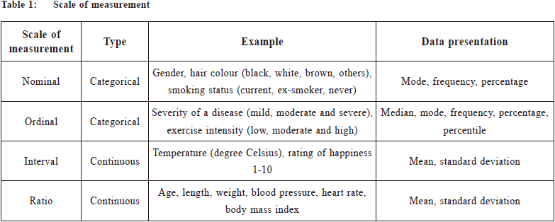

Types of variable - Independent vs dependent variable

To choose a statistical test correctly, the second thing we need to know is what the dependent variables and independent variables are to be analysed in our research. To classify each variable into dependent and independent variables, it depends on the design and outcomes of our research.

Independent variables

Independent variables are variables that can be controlled or determined by researchers in the research. The independent variables can also be called as predictors, explanatory variables and exposure variables. The independent variables are usually used to predict the values of the dependent variables in a statistical model.

Dependent variables

Dependent variables are variables that cannot be controlled or determined by researchers in the research. The dependent variables can also be called as predicted variables and observed variables. In a clinical study, dependent variables are the outcomes that the researchers would like to look into or the outcomes that can answer the research question formulated by the researchers. We look at the difference in the changes in dependent variables in different levels or measurements of independent variables.

For example, we want to find out the factors that can affect intelligence of a student or, in other words, we want to look into the difference in intelligence with the different aspects of variables collected. Therefore, an intelligence score of a student could be a dependent variable because it can be changed depending on several factors, such as the school the student is attending, father and mother intelligence, gender, age, the time the student spent in doing intelligence related exercise or even the sleep quality before he does the intelligence test. All the factors, that we think or have been shown by past literature that can affect the intelligence of a student can be collected and classified as independent variables.

Normal distribution (mean, variance and standard deviation)

Normal distribution is an important concept in doing statistical analysis since many statistical tests are done based on the assumption of normal distribution. If the data is not normally distributed, the choice of statistical tests will be largely reduced. However, we can transform the data to make it normally distributed in some circumstances.

Before we go into normal distribution, we need to understand the concept of population, sample, variance and standard deviation. Population is a complete set of elements (persons or objects). Sample is one or more persons or objects from the population. For example, we conduct a study on a drug effect on lung cancer patients in Hong Kong. The population is all lung cancer patients in Hong Kong and the sample is, say 100, patients in a public hospital. Variance, denoted as σ² for population variance and S² for sample variance, measures how far a data set is spread out. It is defined as “the average of the squared differences from the mean”, which gives you a very general idea of the spread of the data. If every input is the same, the variance is equal to zero which means that there is no variability. Standard deviation, denoted as σ for population standard deviation and S for sample standard deviation, is the square root of the variance.

Normal distribution

A normal distribution (Figure 1) is a distribution of a variable in a bell shape with most of the data in the middle and an equal spread out of data to the left and the right. The middle of value of the normal distribution is equal to the mean, median and mode of the data. Also, around 68%, 95% and 99.5% of the values lie within one, two and three standard deviations of the mean, respectively. Therefore, the value of mean and standard deviation of the data confirm the shape of the normal distribution.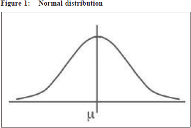

Standard normal distribution is a normal distribution with mean=0 and standard deviation=1. Every data with normal distribution can be transformed into standard normal distribution by deducting the mean of the data and divided by the standard deviation of the data, like the formula below.

Central Limit Theorem

Central Limit Theorem(CLT)² tells us that the distribution of the mean of the data is, at least approximately, normally distributed, regardless of the distribution of the underlying distribution of the data when the data has sufficiently large samples. Usually, sufficiently large means 25-30 samples. When the data is more skewed to the right or the left, more samples are required to make use of CLT. In reality, it is impossible to find a data to follow normal distribution precisely. However, most of the statistical tests have the assumption of normal distribution of the data. Therefore, it is impossible to make use of any statistical tests. However, based on this theorem, we can assume the data mean is approximately normally distributed with a sample more than 25. Therefore, we can make use of most statistical tests with the normal distribution assumption.

Confidence interval

In doing a study, we draw a sample from the population and draw conclusions. Therefore, the mean we get from the sample is not the same as the mean from the population. So, confidence interval, a range of value that we are, for example 95%, confident that the true value is within this range, is established. In other words, when you repeat the same study 100 times targeting the same population, we expect there are 95 times the mean is within this 95% confidence interval.

To construct a confidence interval, for example 95% confidence interval for mean, we require the mean and the standard deviation of the mean by the formula below.

Lower bound: Mean – Z * SD(mean)
Upper bound: Mean + Z * SD(mean)

where, Z=1.96 for 95% confidence interval, SD (mean) = where = S is standard deviation of the sample and n is the number of participant in the sample.

The value of Z will increase when you to have a higher percentage of confidence interval, for example Z=2.24 for 97.5% confidence interval, and decrease when you have a lower percentage of confidence interval, for example Z=1.645 for 90% confidence interval.

For example:

We want to look at the 95% confidence interval of a sample of 100 primary students with an average height of 150cm and the standard deviation of the sample height of 20.

Lower bound: 150 – 1.96 * = 146.08cm, Z=1.96 for 95% confidence interval

Upper bound: 150 + 1.96 * = 153.92cm, Z=1.96 for 95% confidence interval

Conclus ion: We ar e 95% conf ident that the true mean of the studied primary student is between 146.08cm and 153.92cm.

Conclusion

When we make use of statistics to help us draw conclusion, we always need to bear in mind that it is a probability only. We can never be 100% certain to conclude or reject one thing.